1. 线性回归
简述
在统计学中,线性回归(Linear Regression)是利用称为线性回归方程的最小平方函数对一个或多个自变量和因变量之间关系进行建模的一种回归分析。这种函数是一个或多个称为回归系数的模型参数的线性组合(自变量都是一次方)。只有一个自变量的情况称为简单回归,大于一个自变量情况的叫做多元回归。
优点:结果易于理解,计算上不复杂。
缺点:对非线性数据拟合不好。
适用数据类型:数值型和标称型数据。
算法类型:回归算法
线性回归的模型函数如下:
它的损失函数如下:
通过训练数据集寻找参数的最优解,即求解可以得到的参数向量,其中这里的参数向量也可以分为参数,分别表示权重和偏置值。
求解最优解的方法有最小二乘法和梯度下降法。
梯度下降法
梯度下降算法的思想如下(这里以一元线性回归为例):
首先,我们有一个代价函数,假设是,我们的目标是。
接下来的做法是:
首先是随机选择一个参数的组合,一般是设;
然后是不断改变,并计算代价函数,直到一个局部最小值。之所以是局部最小值,是因为我们并没有尝试完所有的参数组合,所以不能确定我们得到的局部最小值是否便是全局最小值,选择不同的初始参数组合,可能会找到不同的局部最小值。
下面给出梯度下降算法的公式:repeat until convergence{
}
也就是在梯度下降中,不断重复上述公式直到收敛,也就是找到。其中符号:=是赋值符号的意思。
而应用梯度下降法到线性回归,则公式如下:
公式中的称为学习率(learning rate),它决定了我们沿着能让代价函数下降程度最大的方向向下迈进的步子有多大。
在梯度下降中,还涉及都一个参数更新的问题,即更新,一般我们的做法是同步更新。
最后,上述梯度下降算法公式实际上是一个叫批量梯度下降(batch gradient descent),即它在每次梯度下降中都是使用整个训练集的数据,所以公式中是带有。
岭回归(ridge regression):
岭回归是一种专用于共线性数据分析的有偏估计回归方法,实质上是一种改良的最小二乘估计法,通过放弃最小二乘法的无偏性,以损失部分信息、降低精度为代价,获得回归系数更为符合实际、更可靠的回归方法,对病态数据的耐受性远远强于最小二乘法。
岭回归分析法是从根本上消除复共线性影响的统计方法。岭回归模型通过在相关矩阵中引入一个很小的岭参数K(1>K>0),并将它加到主对角线元素上,从而降低参数的最小二乘估计中复共线特征向量的影响,减小复共线变量系数最小二乘估计的方法,以保证参数估计更接近真实情况。岭回归分析将所有的变量引入模型中,比逐步回归分析提供更多的信息。
其他回归还可以参考这篇文章。
代码实现
Python实现的代码如下:
#Import Library
#Import other necessary libraries like pandas, numpy...
from
 sklearn
import
 linear_model
#Load Train and Test datasets
#Identify feature and response variable(s) and values must be numeric and numpy arrays
x_train=input_variables_values_training_datasets
y_train=target_variables_values_training_datasets
x_test=input_variables_values_test_datasets
# Create linear regression object
linear = linear_model.LinearRegression()
# Train the model using the training sets and check score
linear.fit(x_train, y_train)
linear.score(x_train, y_train)
#Equation coefficient and Intercept
print(
'Coefficient: \n'
, linear.coef_)
print(
'Intercept: \n'
, linear.intercept_)
#Predict Output
predicted= linear.predict(x_test)
上述是使用sklearn包中的线性回归算法的代码例子,下面是一个实现的具体例子。
# -*- coding: utf-8 -*-
"""
Created on Mon Oct 17 10:36:06 2016

@author: cai
"""
import
 os
import
 numpy
as
 np
import
 pandas
as
 pd
import
 matplotlib.pylab
as
 plt
from
 sklearn
import
 linear_model
# 计算损失函数
def

computeCost
(X, y, theta)
:

    inner = np.power(((X * theta.T) - y),
2
)
return
 np.sum(inner) / (
2
 * len(X))
# 梯度下降算法
def

gradientDescent
(X, y, theta, alpha, iters)
:

    temp = np.matrix(np.zeros(theta.shape))
    parameters = int(theta.ravel().shape[
1
])
    cost = np.zeros(iters)
for
 i
in
 range(iters):
        error = (X * theta.T) - y
for
 j
in
 range(parameters):
# 计算误差对权值的偏导数

            term = np.multiply(error, X[:, j])
# 更新权值

            temp[
0
, j] = theta[
0
, j] - ((alpha / len(X)) * np.sum(term))

        theta = temp
        cost[i] = computeCost(X, y, theta)
return
 theta, cost

dataPath = os.path.join(
'data'
,
'ex1data1.txt'
)
data = pd.read_csv(dataPath, header=
None
, names=[
'Population'
,
'Profit'
])
# print(data.head())
# print(data.describe())
# data.plot(kind='scatter', x='Population', y='Profit', figsize=(12, 8))
# 在数据起始位置添加1列数值为1的数据
data.insert(
0
,
'Ones'
,
1
)
print(data.shape)

cols = data.shape[
1
]
X = data.iloc[:,
0
:cols-
1
]
y = data.iloc[:, cols-
1
:cols]
# 从数据帧转换成numpy的矩阵格式
X = np.matrix(X.values)
y = np.matrix(y.values)
# theta = np.matrix(np.array([0, 0]))
theta = np.matrix(np.zeros((
1
, cols-
1
)))
print(theta)
print(X.shape, theta.shape, y.shape)
cost = computeCost(X, y, theta)
print(
"cost = "
, cost)
# 初始化学习率和迭代次数
alpha =
0.01
iters =
1000
# 执行梯度下降算法
g, cost = gradientDescent(X, y, theta, alpha, iters)
print(g)
# 可视化结果
x = np.linspace(data.Population.min(),data.Population.max(),
100
)
f = g[
0
,
0
] + (g[
0
,
1
] * x)

fig, ax = plt.subplots(figsize=(
12
,
8
))
ax.plot(x, f,
'r'
, label=
'Prediction'
)
ax.scatter(data.Population, data.Profit, label=
'Training Data'
)
ax.legend(loc=
2
)
ax.set_xlabel(
'Population'
)
ax.set_ylabel(
'Profit'
)
ax.set_title(
'Predicted Profit vs. Population Size'
)

fig, ax = plt.subplots(figsize=(
12
,
8
))
ax.plot(np.arange(iters), cost,
'r'
)
ax.set_xlabel(
'Iteration'
)
ax.set_ylabel(
'Cost'
)
ax.set_title(
'Error vs. Training Epoch'
)
# 使用sklearn 包里面实现的线性回归算法
model = linear_model.LinearRegression()
model.fit(X, y)

x = np.array(X[:,
1
].A1)
# 预测结果
f = model.predict(X).flatten()
# 可视化
fig, ax = plt.subplots(figsize=(
12
,
8
))
ax.plot(x, f,
'r'
, label=
'Prediction'
)
ax.scatter(data.Population, data.Profit, label=
'Training Data'
)
ax.legend(loc=
2
)
ax.set_xlabel(
'Population'
)
ax.set_ylabel(
'Profit'
)
ax.set_title(
'Predicted Profit vs. Population Size(using sklearn)'
)
plt.show()
上述代码参考自Part 1 – Simple Linear Regression。具体可以查看我的Github。
2. 逻辑回归
简述
Logistic回归算法基于Sigmoid函数,或者说Sigmoid就是逻辑回归函数。Sigmoid函数定义如下:
。函数值域范围(0,1)。
因此逻辑回归函数的表达式如下:
其导数形式为:
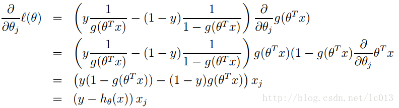
代价函数
逻辑回归方法主要是用最大似然估计来学习的,所以单个样本的后验概率为:
到整个样本的后验概率就是:
其中,。
通过对数进一步简化有:.
而逻辑回归的代价函数就是。也就是如下所示:
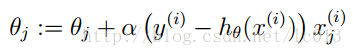
同样可以使用梯度下降算法来求解使得代价函数最小的参数。其梯度下降法公式为:
总结
优点:
1、实现简单;
2、分类时计算量非常小,速度很快,存储资源低;
缺点:
1、容易欠拟合,一般准确度不太高
2、只能处理两分类问题(在此基础上衍生出来的softmax可以用于多分类),且必须线性可分;
适用数据类型:数值型和标称型数据。
类别:分类算法。
试用场景:解决二分类问题。
代码实现
首先是采用sklearn包中的逻辑回归算法代码:
#Import Library
from
 sklearn.linear_model
import
 LogisticRegression
#Assumed you have, X (predictor) and Y (target) for training data set and x_test(predictor) of test_dataset
# Create logistic regression object
model = LogisticRegression()
# Train the model using the training sets and check score
model.fit(X, y)
model.score(X, y)
#Equation coefficient and Intercept
print(
'Coefficient: \n'
, model.coef_)
print(
'Intercept: \n'
, model.intercept_)
#Predict Output
predicted= model.predict(x_test)
接下来则是应用例子,如下所示:
#!/usr/bin/env python# -*- coding: utf-8 -*-"""
@Time    : 2016/10/19 21:35
@Author  : cai

实现多类的逻辑回归算法
"""import osimport numpy as npimport pandas as pdimport matplotlib.pylab as pltfrom scipy.optimize import minimizefrom scipy.io import loadmat# 定义Sigmoid函数def sigmoid(z):
    return 1 / (1 + np.exp(-z))# 定义 cost函数def costReg(theta, X, y, lambdas):
    theta = np.matrix(theta)
    X = np.matrix(X)
    y = np.matrix(y)
    h = X * theta.T
    first = np.multiply(-y, np.log(sigmoid(h)))
    second = np.multiply((1-y), np.log(1 - sigmoid(h)))
    reg = (lambdas / 2 * len(X)) * np.sum(np.power(theta[:, 1:theta.shape[1]], 2))    return np.sum(first - second) / (len(X)) + reg# 梯度下降算法的实现, 输出梯度对权值的偏导数def gradient(theta, X, y, lambdas):
    theta = np.matrix(theta)
    X = np.matrix(X)
    y = np.matrix(y)

    parameters = int(theta.ravel().shape[1])
    grad = np.zeros(parameters)    # 计算误差
    error = sigmoid(X * theta.T) - y

    grad = ((X.T * error) / len(X)).T + ((lambdas / len(X)) * theta)

    grad[0, 0] = np.sum(np.multiply(error, X[:, 0])) / len(X)    return np.array(grad).ravel()# 实现一对多的分类方法def one_vs_all(X, y, num_labels, lambdas):
    rows = X.shape[0]
    params = X.shape[1]    # 每个分类器有一个 k * (n+1)大小的权值数组
    all_theta = np.zeros((num_labels, params + 1))    # 增加一列,这是用于偏置值
    X = np.insert(X, 0, values=np.ones(rows), axis=1)    # 标签的索引从1开始
    for i in range(1, num_labels + 1):
        theta = np.zeros(params + 1)
        y_i = np.array([1 if label == i else 0 for label in y])
        y_i = np.reshape(y_i, (rows, 1))        # 最小化损失函数
        fmin = minimize(fun=costReg, x0=theta, args=(X, y_i, lambdas), method='TNC', jac=gradient)
        all_theta[i-1, :] = fmin.x    return all_thetadef predict_all(X, all_theta):
    rows = X.shape[0]
    params = X.shape[1]
    num_labels = all_theta.shape[0]    # 增加一列,这是用于偏置值
    X = np.insert(X, 0, values=np.ones(rows), axis=1)

    X = np.matrix(X)
    all_theta = np.matrix(all_theta)    # 对每个训练样本计算其类的概率值
    h = sigmoid(X * all_theta.T)    # 获取最大概率值的数组索引
    h_argmax = np.argmax(h, axis=1)    # 数组是从0开始索引,而标签值是从1开始,所以需要加1
    h_argmax = h_argmax + 1

    return h_argmax

dataPath = os.path.join('data', 'ex3data1.mat')# 载入数据data = loadmat(dataPath)
print(data)
print(data['X'].shape, data['y'].shape)# print(np.unique(data['y']))# 测试# rows = data['X'].shape[0]# params = data['X'].shape[1]## all_theta = np.zeros((10, params + 1))## X = np.insert(data['X'], 0, values=np.ones(rows), axis=1)## theta = np.zeros(params + 1)## y_0 = np.array([1 if label == 0 else 0 for label in data['y']])# y_0 = np.reshape(y_0, (rows, 1))# print(X.shape, y_0.shape, theta.shape, all_theta.shape)all_theta = one_vs_all(data['X'], data['y'], 10, 1)
print(all_theta)# 计算分类准确率y_pred = predict_all(data['X'], all_theta)
correct = [1 if a == b else 0 for (a, b) in zip(y_pred, data['y'])]
accuracy = (sum(map(int, correct)) / float(len(correct)))
print('accuracy = {0}%'.format(accuracy * 100))
实现代码来自Part 4 – Multivariate Logistic Regression。具体可以查看我的github 。


评论